NFT Attribute Types: A rarity system (but with Maths)

(Originally posted here)

At this point in time, almost everyone has heard about NFTs. Even if you don’t really understand how they work, you associate them with images of Apes or Cats. Check a couple of them, just for reference:

• Bored Ape Yacht Club
• CryptoKitties
• CryptoPunks

Technically, and also theoretically, NFTs are not just that, but for this blog post, we’ll just stick with profile pictures that have different attributes. If you want to know a bit more in-depth about NFTs in general and other possible applications, go check Francisco’s post, also for the initiates in the area.

What are these attributes, you ask? Well, they are associated with the metadata of the Asset, and in the case of the profile pics, these attributes will define what your final image looks like and create a perceived sense of scarcity (or rarity).

As an example, we will use the Bored Ape owned by our good friend Roberto from Subvisual.

Checking on the metadata, provided by its OpenSea page, this token has the following attributes, and respective rarities:

• Background: blue (12%);
• Clothes: tweed suit (1%);
• Eyes: coins (5%);
• Fur: gray (5%);
• Hat: Faux Hawk (1%);
• Mouth: Phoneme Oh (2%);

How were these percentages calculated? We’ll try to better understand them below, and try to come up with our own way of pre-calculating a rarity for an attribute.

If this got your attention, and you want to know more about how overall rarities are calculated (how someone judges an NFT as rarer than another), go check this post from rarity.tools.

What are we doing and why?⌗

We want to pre-generate the metadata for a set of NFTs that will have several attributes. This metadata has information on the traits of that specific NFT, in this case, each attribute type and the respective value.

For example, if we want to generate the metadata for an NFT that has different types of glasses, the plan is to calculate the total number of tokens that will have round, square, emoji glasses, or even no glasses at all. This will specify the rarity of each attribute type.

The question of how other Buidlers are doing this came up in one of the projects we are currently working at, as Finiam. We assumed right away that they should obey some kind of mathematical rule, defined by the creators, distributing attribute values, for the final image to have a “real” sense of rarity and scarcity… But, there’s also the chance that each attribute value is just licking the finger and sticking it up in the wind.

This way, Resende and I started looking for references and if someone had documented their journey of calculating rarities and how they had done it. We found no evidence that they did have used mathematical distributions, or at least they weren’t open about it at all.

Bored Ape Yacht Club - rarities breakdown⌗

Resende had developed a Jupyter notebook where you can just introduce the URI of the metadata for a certain contract, and then the script creates a dictionary (map) with the overall information of each attribute type.

We decided to inspect the BAYC contract. Looking at their OpenSea collection page, you can see that they have 7 different attributes, and the number of types for each one varies from 6 to 43. For the sake of this blog post, we’ll just show you two of the generated plots. If interested to get more information give us a nudge on Twitter.

The following plots represent a histogram for each attribute type of Clothes and Eyes, respectively.

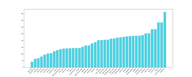
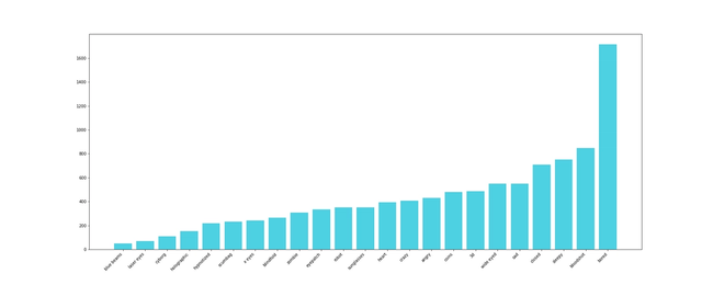
We won’t discuss if they used some mathematical distribution to calculate each amount or if it was eyeballing, but you can try to estimate if this really uses any math as the base.

Getting our hands dirty⌗

After this, for us, it was very simple: “Let’s do it ourselves!” The perfect excuse to finally put in practice those Calculus and Statistics lessons in college that we never got to use, until now!

This way, the goal to develop something interactive to calculate the number of NFTs that will have each type of attribute, was set.

Note: Here it’s also possible to check a statistical analysis on a different type of projects (eg. generative art from Artblocks.io. So if you’re into statistics give it a look also.)

Looking at mathematical distributions and functions⌗

The first step was looking at the plots of some distributions that we already knew and seeing which ones could be adapted into defining a cool rarity system.

We looked into a bunch of them, and to be honest, we don’t remember anymore which ones were. Some weren’t even a distribution, like the sin function, that we also investigated, because of its malleability to have the 0’s where we want them and also for the waving shape. So, as a summary, we’ll only talk about the two that got selected.

Negative Exponential⌗

After our initial brainstorm session, we knew we wanted to use the negative exponential function. Just looking at the plot, it screams rarity system. How? Let’s have a look at the example below.

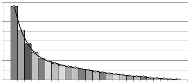
Imagine dividing the area of the negative exponential function (integral in the Wikipedia if you’re not familiar with it) by the number of total attributes we want to calculate a rarity for, just like it is in the image. In that case, we have 25 columns, that would represent 25 different attributes. We get each rarity by calculating the approximate area of each column and dividing it by the total area, thus getting a percentage. This percentage then represents the mathematical distribution and the respective percentage of occurrences for that attribute.

I know I just described how distributions are calculated with Integrals, but the point here is that we get a clear decline of the area of each column, giving us the proportion for each attribute from the most common to the rarest.

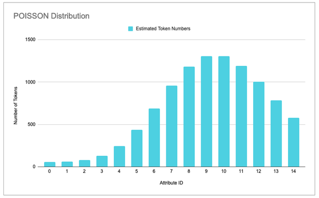
Poisson Distribution⌗

Then, the other option that we also went with is the Poisson distribution, because it has a cool name. Well, not only that but because it offers a very different perspective of the negative exponential and enables more possible combinations of attributes rarity.

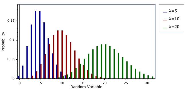
Looking at the image above, you can see what’s that difference I was mentioning. Just looking at the bars you might confuse the Poisson distribution with a Normal distribution, but they are slightly different, and that’s the real reason we chose it.

The Poisson Distribution has a lower bound at 0 and no upper bound, while the Normal Distribution has no bounds at all. Also, unlike a normal distribution, which is always symmetric, the basic shape of a Poisson distribution changes. To know a bit more about these differences check this.

The same mathematical approach with the negative exponential to calculate areas and percentages, also applies here, as with other distributions.

Taking advantage of Google Sheets⌗

We didn’t want to implement these distributions ourselves, despite understanding the maths behind it. So we turn our heads to the good friend Google Sheets that already has a bunch of distributions implemented, and can be used out of the box.

Another good thing about Google Sheets, or any other famous spreadsheet, is that it’s also easily programmable and interactive. We can define cells where we change the inputs, and others displaying results, change accordingly.

And finally, plotting results and conclusions is also effortless, and pretty much necessary for this use case. It’s kinda cool to visualize what different attribute rarities would look like.

Making it dynamic with configurable values⌗

As I hinted earlier, we wanted to do it configurable so we could test different combinations and options with ease.

Two things that we need to be interactive are the number of tokens to be emitted, or in other words, the amount of NFTs that will exist in this collection and the number of different possibilities an attribute will have, so we can calculate the distribution only for those values.

Also, looking at the Poisson Distribution function, we see that it’s also possible to make λ vary. λ must be greater than 0, and it is equal to the expected value of X and also to its variance (variance in Wikipedia). This way, we can have even more combinations and possibilities.

Calculating rarities with Poisson⌗

To calculate rarities with the Poisson distribution we used the function POISSON.DIST(x, mean, [cumulative]) that Google Sheets already provides. Sheets provides more information on it, but basically, in our situation:

• x will be the id of the attribute ranging from 0 to total attributes.
• f will be the mean of the Poisson distribution function (λ).
• [cumulative] is a boolean to identify if we want to use the cumulative distribution function rather than the distribution function (the sum of all columns until the X we are using instead of just the column X, using the same analogy as above).

However, just doing this we have a slight problem… The Poisson Distributed is not bounded to the right of the X-axis, so if we just want to calculate the distribution for a small number of attributes, there’s the chance that the probabilities don’t add up to 100%, because we’re missing some x-values.

Looking at the generated plot above using only the distribution value for 15 different attributes of 10000 tokens (NFTs), and with a mean value of 10, we see that some values are missing to the right, and if we add all of the probabilities we get just 91.65%. The rest 8.35% are for values of X above 15, which we don’t want. The objective is if we have only 15 attributes, the sum of their probabilities must be 100%.

So the solution we came up with is calculating the missing percentage to 100% and dividing it by the number of attributes, and adding this part to each attribute. Using the example above, we would divide the 8.35% that is missing by 15 (equating to approximately 0.56%), and add this value to each existing column, therefore spreading this exceed evenly.

The final formula is this, using the cumulative version to actually obtain the exceeding probabilities to the right of the function.

POISSON.DIST(x, mean, false) + ((1 - POISSON.DIST(totalAttributes - 1, mean, true)) / totalAttributes)

Below, we have the updated version, and if we compare the two plots, we see that now the first attributes have a probability different than 0, because we are also taking into account the exceeding values, and the sum of all of them is equal to 100% or the total number of tokens to be created.

Calculating rarities with Negative Exponential⌗

For the negative exponential distribution, we used the function EXPONDIST(x, lambda, [cumulative]).

• x will be the id of the attribute raging from 0 to total attributes.
• lambda is the parameter of the distribution, often called the rate parameter.
• [cumulative] represents the same as in the Poisson one.

In this case, we are leaving the lambda fixed as 1, for simplicity. This distribution was a bit more complicated to get around so we went with the shortest path to having anything providing correct results.

The first problem arose from the idea of dividing the function into columns. This process was not that direct, as in the Poisson case. The formula we arrived at to have a proper result, is the following:

EXPONDIST((4.60517 / totalAttributes) * X, 1, false)  - EXPONDIST((4.60517 / totalAttributes) * (X + 1), 1, false)

Why the subtraction, and why that 4.60517?? First, let’s have look at the “strange” value and we got it.

The value (~4.6) comes from solving the following expression of - (ln (1 - 0.99)). This is obtained from the integral of the negative exponential function e^-x and trying to obtain the X value where the area of the function is approximately 0.99. If you want to check the step-by-step solution, have a look at this Wolfram solution for it. Following the same approach, we can divide it into smaller columns and get the relative proportion. But why 0.99? As this function tends to 1 at the infinity, we chose to use 99% as the full area, otherwise, percentages for the rarest attributes would be basically 0.

Returning to the expression above (4.60517 / totalAttributes) * X we divide the area by the number of attributes and multiply it by the value of X we are calculating at the time, simulating the column divisions referenced above.

The same issue with boundaries that happened in the Poisson Distribution also happens here, so we used the same solution. Calculate the exceeding values, and add them evenly to each attribute percentage.

This way both distributions may not produce the values as they would in normal mathematical conditions, as they were adapted to fit this very specific problem with a discrete number of variables. Note: we are not mathematicians so we are sure that there is some obscure way of doing the same thing but mathematically correct.

How do we use this for tangible information?⌗

The final question is how we retrieve the actual number of tokens that will have each type of attribute. For that, we decide to do a quick demo.

In the video above, we set the number of tokens to 1000 and 5 different attributes (where we set some fake attribute names just to help identify stuff in the long run), and then the mean value of the Poisson Distribution to 3 (basically setting the most common id). It’s also possible to see how the cells and plots change when we change the different configurable values.

Red columns represent the actual number of tokens that we want for a specific attribute, based on the predictions given by the distribution we choose, as they produce decimal values that can’t be applied to our use case (a token must be a full unit).

Final thoughts⌗

Looking back at this experience, there’s a slight chance that the solution was a bit of over-engineering, but it was the perfect opportunity to put this knowledge to the test.

We hope you have liked this approach to rarities in NFTs, and feel free to reach out if you want to know more about this spreadsheet.

Have a nice one and see you in the next blogpost 👋